2. Background Theory

This section aims to provide the user with a basic review of the physics, discretization, and optimization techniques used to solve the time domain electromagnetics problem. It is assumed that the user has some background in these areas. For further reading see [Nab91].

2.1. Fundamental Physics

Maxwell’s equations provide the starting point from which an understanding of how electromagnetic fields can be used to uncover the substructure of the Earth. The time domain Maxwell’s equations are:

(2.1)\[\begin{split}\nabla \times & \vec{e} = - \partial_t \vec{b} \\ \nabla \times & \vec{h} - \vec{j} = \vec{s} \, f(t) \\ \vec{j} &= \sigma \vec{e} \\ \vec{b} &= \mu \vec{h}\end{split}\]

where \(\vec{e}\), \(\vec{h}\), \(\vec{j}\) and \(\vec{b}\) are the electric field, magnetic field, current density and magnetic flux density, respectively. \(\vec{s}\) contains the geometry of the source term and \(f(t)\) is a time-dependent waveform. Symbols \(\mu\) and \(\sigma\) represent the magnetic permeability and electrical conductivity, respectively. This formulation assumes a quasi-static mode so that the system can be viewed as a diffusion equation (Weaver, 1994; Ward and Hohmann, 1988 in Nabighian, 1991`. By doing so, some difficulties arise when solving the system;

• the electrical conductivity \(\sigma\) varies over several orders of magnitude

• the fields can vary significantly near the sources, but smooth out at distance thus high resolution is required near sources

2.2. Octree Mesh

By using an Octree discretization of the earth domain, the areas near sources and likely model location can be give a higher resolution while cells grow large at distance. In this manner, the necessary refinement can be obtained without added computational expense. The figure below shows an example of an Octree mesh, with nine cells, eight of which are the base mesh minimum size.

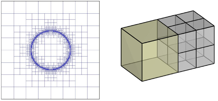
When working with Octree meshes, the underlying mesh is defined as a regular 3D orthogonal grid where the number of cells in each dimension are \(2^{n_1} \times 2^{n_2} \times 2^{n_3}\). The cell widths for the underlying mesh are \(h_1, \; h_2, \; h_3\), respectively. This underlying mesh is the finest possible, so that larger cells have side lengths which increase by powers of 2. The idea is that if the recovered model properties change slowly over a certain volume, the cells bounded by this volume can be merged into one without losing the accuracy in modeling, and are only refined when the model begins to change rapidly.

2.3. Discretization of Operators

The operators div, grad, and curl are discretized using a finite volume formulation. Although div and grad do not appear in (2.1) , they are required for the solution of the system. The divergence operator is discretized in the usual flux-balance approach, which by Gauss’ theorem considers the current flux through each face of a cell. The nodal gradient (operates on a function with values on the nodes) is obtained by differencing adjacent nodes and dividing by edge length. The discretization of the curl operator is computed similarly to the divergence operator by utilizing Stokes theorem by summing the magnetic field components around the edge of each face. Please see Haber (2012) for a detailed description of the discretization process.

2.4. Forward Problem

2.4.1. Initial Conditions

To solve for the first time step using direct or iterative methods, we will need to first solve for the electric fields at \(t=t_0\). Assuming the source is static for \(t \leq t_0\), (2.1) reduces to:

(2.2)\[\begin{split}\nabla \cdot \vec{j} &= - f_0 \, \nabla \cdot \vec{s} \\ \vec{j} &= \sigma \vec{e} \\ \vec{e} &= \nabla \phi\end{split}\]

where \(\vec{j}\) is the current density, \(\phi\) is the scalar potential and \(f_0\) is the waveform at \(t \leq t_0\). By applying the finite volume method, the static electric fields are obtained by solving the following system:

(2.3)\[\big [ \mathbf{G^T \, N_e^T \, M_\sigma \, N_e \, G} \big ] \, \phi_0 = -f_0 \, \mathbf{G^T \, s_j}\]

where \(\phi_0\) lives on nodes, \(\mathbf{s_j}\) defines the geometry of the source (as a current density) discretized to the mesh and

(2.4)\[\begin{split}\mathbf{M_\sigma} &= diag \big ( \mathbf{A^T_{e2c} V} \, \boldsymbol{\sigma} \big ) \\ \mathbf{G} &= \mathbf{P_n \, \tilde G \, N_n}\end{split}\]

\(\mathbf{V}\) is a diagonal matrix containing all cell volumes, and \(\mathbf{A_{e2c}}\) averages from edges to cell centres. The conductivity for each cell is contained within the vector \(\boldsymbol{\sigma}\). The matrix \(\mathbf{N_e}\) provides edge constraints which address inaccuracies associated with ‘hanging edges’ in the OcTree mesh. The matrix \(\mathbf{N_n}\) provides nodal constraints which address inaccuracies associated with ‘hanging nodes’ in the OcTree mesh. \(\mathbf{P_n}\) is a projection matrix. \(\mathbf{\tilde G}\) is the gradient operator, thus \(\mathbf{G}\) is a modified gradient operator.

Once obtained, the electric field on cell edges at \(t=t_0\) is obtained via:

(2.5)\[\mathbf{e_0} = \mathbf{G \, \phi_0}\]

Note

Equation (2.3) must be solved for each source. However, LU factorization is used to make solving for many right-hand sides more efficient.

2.4.2. Direct Solver Approach

To solve the forward problem (2.1) , we must first discretize in space and then in time. Using finite volume approach, the electric fields on cell edges (\(\mathbf{e}\)) discretized in space are described by:

(2.6)\[\mathbf{C^T \, M_\mu \, C \, e} + \mathbf{N_e^T \, M_\sigma \, N_e} \, \partial_t \mathbf{e} = - \mathbf{s} \, \partial_t f\]

where \(\mathbf{M_\sigma}\) and \(\mathbf{N_e}\) were defined in (2.3), and

(2.7)\[\begin{split}\mathbf{M_\mu} &= diag \big ( \mathbf{A^T_{f2c} V} \, \boldsymbol{\mu^{-1}} \big ) \\ \mathbf{C} &= \mathbf{\tilde C \, N_e}\end{split}\]

\(\mathbf{A_{f2c}}\) averages from faces to cell centres. The inverse magnetic permeability for each cell is contained within the vector \(\boldsymbol{\mu}\). \(\mathbf{\tilde C}\) is the curl operator and \(\mathbf{C}\) is a modified curl operator.

Discretization in time is performed using backward Euler. Thus for a single transmitter, we must solve the following for every time step \(\Delta t_i\):

(2.8)\[\mathbf{A_i \, e_{k+1}} = \mathbf{-B_i \, e_k} + \mathbf{q_i}\]

where

(2.9)\[\begin{split}\mathbf{A_i} &= \mathbf{C^T \, M_\mu \, C } + \Delta t_i^{-1} \mathbf{N_e^T \, M_\sigma \, N_e} \\ \mathbf{B_i} &= - \Delta t_i^{-1} \mathbf{N_e^T \, M_\sigma \, N_e} \\ \mathbf{q_i} &= - \Delta t_i^{-1} \mathbf{N_e^T \, s} \big [ f_{k+1} - f_k \big ]\end{split}\]

Now let \(\mathbf{A_{dc}}\) and \(\mathbf{q_{dc}}\) define the matrix and right-hand side in (2.3) . The forward problem can be expressed as:

(2.10)\[\begin{split}\begin{bmatrix} \mathbf{A_{dc}} & & & & & \\ \mathbf{B_1 \, G} & \mathbf{A_1} & & & & \\ & \mathbf{B_2} & \mathbf{A_2} & & & \\ & & & \ddots & & \\ & & & & \mathbf{B_n} & \mathbf{A_n} \end{bmatrix} \begin{bmatrix} \phi_0 \\ \mathbf{e_1} \\ \mathbf{e_2} \\ \vdots \\ \mathbf{e_n} \end{bmatrix} = \begin{bmatrix} \mathbf{q_{dc}} \\ \mathbf{q_1} \\ \mathbf{q_2} \\ \vdots \\ \mathbf{q_n} \end{bmatrix}\end{split}\]

Note

This problem must be solved for each source. However, LU factorization for each unique time step length is used to make solving for many right-hand sides more efficient.

2.4.3. Iterative Solver Approach

For this approach we decompose the electric field according to the Helmholtz decomposition:

(2.11)\[\vec{e} = \vec{a} + \nabla \phi\]

After formulating Maxwell’s equations in terms of \(\vec{a}\) and \(\phi\), discretizing in space according to the finite volume method and discretizing in time according to backward Euler, we must solve the following numerical system at each time step \(\Delta t_i\):

(2.12)\[\begin{split}\begin{bmatrix} \mathbf{A_i} + \mathbf{D} & - \mathbf{B_i \, G} \\ - \mathbf{G^T \, B_i} & \Delta t_i \, \mathbf{G^T \, B_i \, G} \end{bmatrix} \begin{bmatrix} \mathbf{a_i} \\ \phi_i \end{bmatrix} = \begin{bmatrix} \mathbf{b_i} \\ \mathbf{G^T \, b_i} \end{bmatrix}\end{split}\]

where \(\mathbf{a_i}\) is the vector potential on edges, \(\phi_i\) is the scalar potential on nodes, \(\mathbf{G}\) is the modified gradient operator given by (2.4) and

\[\begin{split}\mathbf{D} &= \mathbf{G} \, diag \big ( \mathbf{A^T_{n2c} V} \, \boldsymbol{\mu^{-1}} \big ) \mathbf{G^T} \\ \mathbf{b_i} &= \mathbf{q_i - B_i \, e_k}\end{split}\]

The matrix \(\mathbf{N_n}\) provides nodal constraints which address inaccuracies associated with ‘hanging nodes’ in the OcTree mesh. \(\mathbf{P_n}\) is a projection matrix. And \(\mathbf{\tilde G}\) is the gradient operator. \(\mathbf{D}\) is a matrix that is added to the (1,1) block of Eq. (2.12) to improve the stability of the system. \(\mathbf{A_i}\), \(\mathbf{B_i}\) and \(\mathbf{q_i}\) are defined in (2.9) .

Once (2.12) is solved, the electric fields on cell edges can be computed numerically according to:

\[\mathbf{e_i} = \mathbf{a_i} + \mathbf{G \, \phi_i}\]

To solve (2.12) we use a block preconditionned conjugate gradient algorithm. For the preconditionner, we do 2 SSOR iterations of (2.12) . Adjustable parameters for solving Eq. (2.12) iteratively using BiCGstab are defined as follows:

• tol_bicg: relative tolerance (stopping criteria) when solver is used during forward modeling; i.e. solves Eq. (2.6) . Ideally, this number is very small (~1e-10).

• tol_ipcg_bicg: relative tolerance (stopping criteria) when solver needed in computation of \(\delta m\) during Gauss Newton iteration; needed to solve Eq. (2.21) . This value does not need to be as large as the previous parameter (~1e-5).

• max_it_bicg: maximum number of BICG iterations (~100)

Note

This problem must be solved for each source.

2.4.4. Magnetic Field at t0

When computing magnetic field data (not needed for \(\vec{e}\) or \(\partial_t \vec{b}\)), we will need to compute magnetic fields at \(t=t_0\). Assuming the source is static for \(t \leq t_0\), (2.1) can be reformulated in terms of a vector potential \(\vec{a}\) and a scalar potential \(\phi\):

\[\begin{split}\nabla \times \mu_{-1} \times \vec{a} + \nabla \mu^{-1} \nabla \cdot \vec{a} &= \sigma \nabla \phi + \vec{s}\, f_0 \\ \vec{b} &= \nabla \times \vec{a} \\ \vec{e} &= \nabla \phi\end{split}\]

where the second term is added for stability assuming the Coulomb Gauge (\(\nabla \cdot \vec{a} = 0\)) condition holds. Using the finite volume approach, we can solve for the discrete vector potential \(\mathbf{a_0}\):

\[\mathbf{A_{m} \, a_0} = \mathbf{q_m}\]

where \(\mathbf{a_0}\) lives on edges and

\[\begin{split}\mathbf{A_{m}} &= \mathbf{C^T \, M_\mu \, C + G \, N_n^T }\, diag \big ( \mathbf{A^T_{n2c} V} \, \boldsymbol{\mu^{-1}} \big ) \mathbf{N_n \, G^T} \\ \mathbf{q_{m}} &= \mathbf{s} \, f_0 + \mathbf{M_\sigma G \, e_0}\end{split}\]

Once we solve for \(\mathbf{a_0}\), the magnetic field is computed via:

\[\mathbf{b_0} = \mathbf{C \, a_0}\]

where \(\mathbf{C}\) is define in (2.7) .

Note

This problem must be solved for each source. However, LU factorization is used to make solving for many right-hand sides more efficient.

2.5. Data

2.5.1. Electric Field

The electric field on cell edges at each time step (\(\mathbf{e_i}\)) is computed using direct or iterative methods. \(\mathbf{Q_e}\) is time-independent linear operator that acts on \(\mathbf{e_i}\). It integrates the electric field at the particular over the length of the receiver wire then divides by its length. The data are therefore the average electric field value over the length of the wire path in units V/m.

The measured electric field for time step \(i\) is given by:

(2.13)\[\mathbf{d_i} = \mathbf{Q_e \, N_e \, e_i}\]

where \(\mathbf{N_e}\) was defined in expression (2.3). Linear interpolation is then used to compute the data for the correct time channel from values defined at each time step.

2.5.2. Time-Derivative of Magnetic Flux

The electric field on cell edges at each time step (\(\mathbf{e_i}\)) is computed using direct or iterative methods. \(\mathbf{Q_b}\) is a time-independent linear operator that acts on \(\mathbf{e_i}\). The operator

• integrates the electric field over path of the receiver loop

• multiplies by -1

• then normalizes by the area of the loop

By Faraday’s law, this results in a computation of average value of dB/dt through the loop in units of T/s. For time step \(i\), the dB/dt measurement at the receiver is given by:

(2.14)\[\mathbf{d_i} = \mathbf{Q_b \, N_e \, e_i}\]

where \(\mathbf{N_e}\) was defined in expression (2.3). Linear interpolation is then used to compute the data for the correct time channel from values defined at each time step.

2.5.3. H-Field

The electric field on cell edges at each time step (\(\mathbf{e_i}\)) is computed using direct or iterative methods. The magnetic flux density (\(\mathbf{b_0}\)) at \(t=t_0\) is computed by solving an a-phi system. Where \(\mathbf{Q_h}\) is a linear operator that projects \(\mathbf{b_0}\) from cell faces to the location of the receiver, the H-field value at \(t=t_0\) is:

\[\mathbf{d_0} = \mu_0^{-1} \, \mathbf{Q_h \, b_0}\]

For subsequent time-steps, the H-field data are computed according to:

(2.15)\[\mathbf{d_i} = \mathbf{d_{i-1}} - \mu_0^{-1} \Delta t_i \, \mathbf{Q_b \, N_e \, e_i}\]

where the term \(\mathbf{Q_b \, N_e \, e_i}\) is equivalent to the dB/dt value at time-step \(i\) according to equation (2.14). Once computed at all time-steps, linear interpolation is then used to compute the data for the correct time channel. The data represent the average magnetic field value through the loop in units A/m.

2.6. Sensitivity

This page is under construction. Have suggestions or want to contribute? Get in touch!

2.7. Inverse Problem

We are interested in recovering the conductivity distribution for the Earth. However, the numerical stability of the inverse problem is made more challenging by the fact rock conductivities can span many orders of magnitude. To deal with this, we define the model as the log-conductivity for each cell, e.g.:

\[\mathbf{m} = log (\boldsymbol{\rho})\]

The inverse problem is solved by minimizing the following global objective function with respect to the model:

(2.16)\[\phi (\mathbf{m}) = \phi_d (\mathbf{m}) + \beta \phi_m (\mathbf{m})\]

where \(\phi_d\) is the data misfit, \(\phi_m\) is the model objective function and \(\beta\) is the trade-off parameter. The data misfit ensures the recovered model adequately explains the set of field observations. The model objective function adds geological constraints to the recovered model. The trade-off parameter weights the relative emphasis between fitting the data and imposing geological structures.

2.7.1. Data Misfit

Here, the data misfit is represented as the L2-norm of a weighted residual between the observed data (\(d_{obs}\)) and the predicted data for a given conductivity model \(\boldsymbol{\sigma}\), i.e.:

(2.17)\[\phi_d = \frac{1}{2} \big \| \mathbf{W_d} \big ( \mathbf{d_{obs}} - \mathbb{F}[\boldsymbol{\sigma}] \big ) \big \|^2\]

where \(W_d\) is a diagonal matrix containing the reciprocals of the uncertainties \(\boldsymbol{\varepsilon}\) for each measured data point, i.e.:

\[\mathbf{W_d} = \textrm{diag} \big [ \boldsymbol{\varepsilon}^{-1} \big ]\]

Important

For a better understanding of the data misfit, see the GIFtools cookbook .

2.7.2. Model Objective Function

Due to the ill-posedness of the problem, there are no stable solutions obtained by freely minimizing the data misfit, and thus regularization is needed. The regularization uses penalties for both smoothness, and likeness to a reference model \(m_{ref}\) supplied by the user. The model objective function is given by:

(2.18)\[\begin{split}\phi_m = \frac{\alpha_s}{2} \!\int_\Omega w_s | m - & m_{ref} |^2 dV + \frac{\alpha_x}{2} \!\int_\Omega w_x \Bigg | \frac{\partial}{\partial x} \big (m - m_{ref} \big ) \Bigg |^2 dV \\ &+ \frac{\alpha_y}{2} \!\int_\Omega w_y \Bigg | \frac{\partial}{\partial y} \big (m - m_{ref} \big ) \Bigg |^2 dV + \frac{\alpha_z}{2} \!\int_\Omega w_z \Bigg | \frac{\partial}{\partial z} \big (m - m_{ref} \big ) \Bigg |^2 dV\end{split}\]

where \(\alpha_s, \alpha_x, \alpha_y\) and \(\alpha_z\) weight the relative emphasis on minimizing differences from the reference model and the smoothness along each gradient direction. And \(w_s, w_x, w_y\) and \(w_z\) are additional user defined weighting functions.

An important consideration comes when discretizing the regularization onto the mesh. The gradient operates on cell centered variables in this instance. Applying a short distance approximation is second order accurate on a domain with uniform cells, but only \(\mathcal{O}(1)\) on areas where cells are non-uniform. To rectify this a higher order approximation is used (Haber, 2012). The second order approximation of the model objective function can be expressed as:

\[\phi_m (\mathbf{m}) = \mathbf{\big (m-m_{ref} \big )^T W^T W \big (m-m_{ref} \big )}\]

where the regularizer is given by:

(2.19)\[\begin{split}\mathbf{W^T W} =& \;\;\;\;\alpha_s \textrm{diag} (\mathbf{w_s \odot v}) \\ & + \alpha_x \mathbf{G_x^T} \textrm{diag} (\mathbf{w_x \odot v_x}) \mathbf{G_x} \\ & + \alpha_y \mathbf{G_y^T} \textrm{diag} (\mathbf{w_y \odot v_y}) \mathbf{G_y} \\ & + \alpha_z \mathbf{G_z^T} \textrm{diag} (\mathbf{w_z \odot v_z}) \mathbf{G_z}\end{split}\]

The Hadamard product is given by \(\odot\), \(\mathbf{v_x}\) is the volume of each cell averaged to x-faces, \(\mathbf{w_x}\) is the weighting function \(w_x\) evaluated on x-faces and \(\mathbf{G_x}\) computes the x-component of the gradient from cell centers to cell faces. Similarly for y and z.

If we require that the recovered model values lie between \(\mathbf{m_L \preceq m \preceq m_H}\) , the resulting bounded optimization problem we must solve is:

(2.20)\[\begin{split}&\min_m \;\; \phi_d (\mathbf{m}) + \beta \phi_m(\mathbf{m}) \\ &\; \textrm{s.t.} \;\; \mathbf{m_L \preceq m \preceq m_H}\end{split}\]

A simple Gauss-Newton optimization method is used where the system of equations is solved using ipcg (incomplete preconditioned conjugate gradients) to solve for each G-N step. For more information refer again to Haber (2012) and references therein.

2.7.3. Inversion Parameters and Tolerances

2.7.3.1. Cooling Schedule

Our goal is to solve Eq. (2.20) , i.e.:

\[\begin{split}&\min_m \;\; \phi_d (\mathbf{m}) + \beta \phi_m(\mathbf{m - m_{ref}}) \\ &\; \textrm{s.t.} \;\; \mathbf{m_L \leq m \leq m_H}\end{split}\]

but how do we choose an acceptable trade-off parameter \(\beta\)? For this, we use a cooling schedule. This is described in the GIFtools cookbook . The cooling schedule can be defined using the following parameters:

• beta_max: The initial value for \(\beta\)

• beta_factor: The factor at which \(\beta\) is decrease to a subsequent solution of Eq. (2.20)

• beta_min: The minimum \(\beta\) for which Eq. (2.20) is solved before the inversion will quit

• Chi Factor: The inversion program stops when the data misfit \(\phi_d \leq N \times Chi \; Factor\), where \(N\) is the number of data observations

2.7.3.2. Gauss-Newton Update

For a given trade-off parameter (\(\beta\)), the model \(\mathbf{m}\) is updated using the Gauss-Newton approach. Because the problem is non-linear, several model updates may need to be completed for each \(\beta\). Where \(k\) denotes the Gauss-Newton iteration, we solve:

(2.21)\[\mathbf{H}_k \, \mathbf{\delta m}_k = - \nabla \phi_k\]

using the current model \(\mathbf{m}_k\) and update the model according to:

(2.22)\[\mathbf{m}_{k+1} = \mathbf{m}_{k} + \alpha \mathbf{\delta m}_k\]

where \(\mathbf{\delta m}_k\) is the step direction, \(\nabla \phi_k\) is the gradient of the global objective function, \(\mathbf{H}_k\) is an approximation of the Hessian and \(\alpha\) is a scaling constant. This process is repeated until any of the following occurs:

1. The gradient is sufficiently small, i.e.:

\[\| \nabla \phi_k \|^2 < tol \_ nl\]

2. The smallest component of the model perturbation its small in absolute value, i.e.:

\[\textrm{max} ( |\mathbf{\delta m}_k | ) < mindm\]

3. A max number of GN iterations have been performed, i.e.

\[k = iter \_ per \_ beta\]

2.7.3.3. Gauss-Newton Solve

Here we discuss the details of solving Eq. (2.21) for a particular Gauss-Newton iteration \(k\). Using the data misfit from Eq. (2.17) and the model objective function from Eq. (2.19), we must solve:

(2.23)\[\Big [ \mathbf{J^T W_d^T W_d J + \beta \mathbf{W^T W}} \Big ] \mathbf{\delta m}_k = - \Big [ \mathbf{J^T W_d^T W_d } \big ( \mathbf{d_{obs}} - \mathbb{F}[\mathbf{m}_k] \big ) + \beta \mathbf{W^T W m}_k \Big ]\]

where \(\mathbf{J}\) is the sensitivity of the data to the current model \(\mathbf{m}_k\). The system is solved for \(\mathbf{\delta m}_k\) using the incomplete-preconditioned-conjugate gradient (IPCG) method. This method is iterative and exits with an approximation for \(\mathbf{\delta m}_k\). Let \(i\) denote an IPCG iteration and let \(\mathbf{\delta m}_k^{(i)}\) be the solution to (2.23) at the \(i^{th}\) IPCG iteration, then the algorithm quits when:

1. the system is solved to within some tolerance and additional iterations do not result in significant increases in solution accuracy, i.e.:

   \[\| \mathbf{\delta m}_k^{(i-1)} - \mathbf{\delta m}_k^{(i)} \|^2 / \| \mathbf{\delta m}_k^{(i-1)} \|^2 < tol \_ ipcg\]

2. a maximum allowable number of IPCG iterations has been completed, i.e.:

   \[i = max \_ iter \_ ipcg\]

2.8. Sensitivity Weights

Sensitivity weights are used to counteract common artifacts associated with TDEM inversion; e.g. ring artifacts observed in the inversion of airborne TDEM data. To construct an appropriate sensitivity weights model, we begin by computing the root mean squared sensitivities. Where n is the number of data and \(v_j\) is the volume of cell \(j\), the root mean squared sensitivity of cell \(j\) is given by:

\[s_j = \frac{1}{v_j} \Bigg [ \sum_{i=1}^n J_{i,j}^2 \; \Bigg ]^{1/2} = \frac{1}{v_j} \Bigg [ diag(\mathbf{J^T J})_j \, \Bigg ]^{1/2}\]

Thus to compute root mean squared sensitivities for all cells, we must compute the diagonal elements of \(\mathbf{J^T J}\). Once obtained, the diagonal elements can be divided by their corresponding cell volumes. We approximate the diagonal elements of \(\mathbf{J^T J}\) iteratively using the probing method:

\[diag( \mathbf{J^T J}) = \frac{1}{K} \sum_{k=1}^K diag (\mathbf{u}) \mathbf{J^T J u}\]

where \(\mathbf{u}\) is a random probing vector and the accuracy of the approximation improves as K increases. The probing method is easy to implement since we have sub-routines for computing the products of \(\mathbf{J}\) and \(\mathbf{J^T}\) with a vector.

The root mean squared sensitivities defined on the mesh are small in magnitude and span many orders of magnitude. To create practical sensitivity weights, the root mean squared sensitivities must be normalized and truncated. This process is explained as follows.

For a vector of root mean squared sensitivities \(\mathbf{s}\), and a maximum sensitivity weight value of \(\tau > 1\), the sensitivity weights are obtained by:

1. normalizing \(\mathbf{s}\) by its maximum value

2. multiplying the resulting vector by \(\tau\)

3. all values less than 1 are set to equal 1