3.2.5. Inversion Input File

The inverse problem is solved using the executable program tdoctree.exe. The lines of input file are as follows:

Line #	Description	Description
1	OcTree Mesh	path to octree mesh file
2	Observation File	path to observations/survey file
3	Transmitter options	discretization options for transmitters
4	Wave file	sets time steps for the time-dependent problem
5	Initial/FWD Model	initial/forward model
6	Reference Model	reference model
7	Susceptibility model	susceptibility model
8	Active Topography Cells	topography
9	Active Model Cells	active model cells
10	Cell Weights	additional cell weights
11	Face Weights	additional face weights
12	beta_max beta_min beta_factor	cooling schedule for beta parameter
13	alpha_s alpha_x alpha_y alpha_z	weighting constants for smallness and smoothness constraints
14	Chi Factor	stopping criteria for inversion
15	iter_per_beta nbetas	set the number of Gauss-Newton iteration for each beta value
16	tol_ipcg max_iter_ipcg	set the tolerance and number of iterations for Gauss-Newton solve
17	Reference Model Update	reference model
18	Hard Constraints	use SMOOTH_MOD or SMOOTH_MOD_DIFF
19	Bounds	upper and lower bounds for recovered model
20	huber_c	Huber constant (for sparse model recovery)
21	Time Channel Indecies	chooses time channels to be inverted

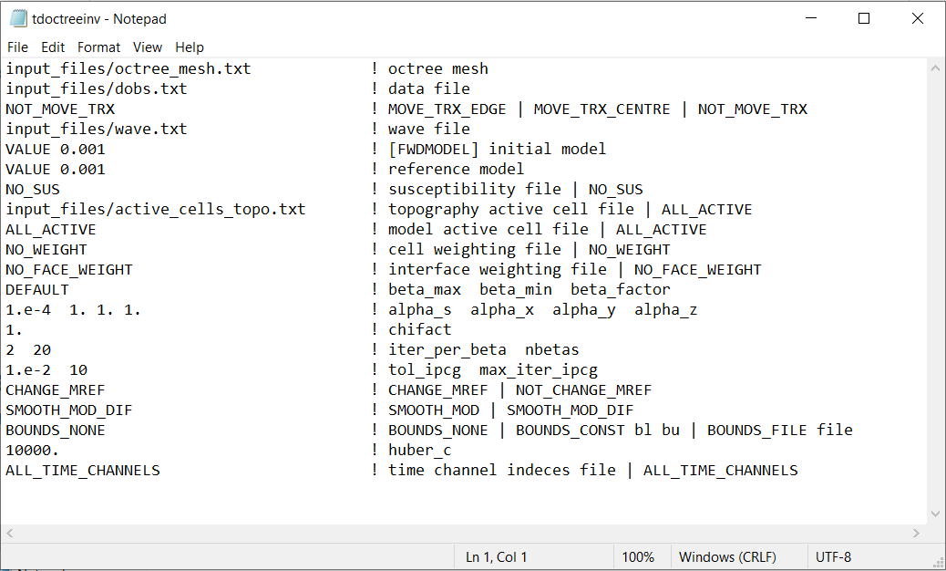
Fig. 3.4 Example input file for the inversion program (Download ). Example input file for forward modeling only (Download ).

3.2.5.1. Line Descriptions

• OcTree Mesh: file path to the OcTree mesh file

• Observation File: file path to the observed data file or a survey file (forward modeling only).

• Transmitter Options: On this line, we can change some aspects as to how the transmitter is discretized to the mesh. There are 3 flags that can be entered:

  • MOVE_TRX_EDGE: Discretizes the transmitters to the nearest edge. Useful for large loop transmitters

  • MOVE_TRX_CENTER: Discretizes the transmitters to the nearest cell center. Useful for dipole transmitters

  • NOT_MOVE_TRX: Do no move the location of transmitters. Keep same as in survey file

• Wave file: Set the path to a wave file. This file defines the time-steps for the problem.

• Initial/FWD Model: On this line we specify either the starting model for the inversion or the conductivity model for the forward modeling. On this line, there are 3 possible options:

  • If the program is being used to forward model data, the flag ‘FWDMODEL’ is entered followed by the path to the conductivity model.

  • If the program is being used to invert data, only the path to a conductivity model is required; e.g. inversion is assumed unless otherwise specified.

  • If a homogeneous conductivity value is being used as the starting model for an inversion, the user can enter “VALUE” followed by a space and a numerical value; example “VALUE 0.01”.

Important

If data are only being forward modeled, only the active topography cells and tol_ipcg max_iter_ipcg fields are relevant. However, the remaining fields must not be empty and must have correct syntax for the code to run.

• Reference Model: The user may supply the file path to a reference conductivity model. If a homogeneous conductivity value is being used for all active cells, the user can enter “VALUE” followed by a space and a numerical value; example “VALUE 0.01”.

• Susceptibility Model: The user may supply the file path to a background susceptibility model. If a homogeneous conductivity value is being used for all active cells, the user can enter “VALUE” followed by a space and a numerical value; example “VALUE 0.01”.

Important

Modeling non-zero susceptibility is possible using the TD OcTree v1 package. However , the initial magnetostatic problem is very difficult to solve for a non-zero transmitter current with our choice in discretization. To model with non-zero susceptibility, you must discretize the entire transmitter waveform and it must start with a current amplitude of 0 at \(t=t_0\) !!!

• Active Topography Cells: Here, the user can choose to specify the cells which lie below the surface topography. To do this, the user may supply the file path to an active cells model file or type “ALL_ACTIVE”. The active cells model has values 1 for cells lying below the surface topography and values 0 for cells lying above.

• Active Model Cells: Here, the user can choose to specify the model cells which are active during the inversion. To do this, the user may supply the file path to an active cells model file or type “ALL_ACTIVE”. The active cells model has values 1 for cells lying below the surface topography and values 0 for cells lying above. Values for inactive cells are provided by the background conductivity model.

• Cell Weights: Here, the user specifies whether cell weights are supplied. If so, the user provides the file path to a cell weights file If no additional cell weights are supplied, the user enters “NO_WEIGHT”.

• Face Weights: Here, the user specifies whether face weights are supplied. If so, the user provides the file path to a face weights file cell weights file. If no additional cell weights are supplied, the user enters “NO_FACE_WEIGHT”. The user may also enter “EKBLOM” for 1-norm approximation to recover sharper edges.

• beta_max beta_min beta_factor: Here, the user specifies protocols for the trade-off parameter (beta). beta_max is the initial value of beta, beta_min is the minimum allowable beta the program can use before quitting and beta_factor defines the factor by which beta is decreased at each iteration; example “1E4 10 0.2”. The user may also enter “DEFAULT” if they wish to have beta calculated automatically.

• alpha_s alpha_x alpha_y alpha_z: Alpha parameters . Here, the user specifies the relative weighting between the smallness and smoothness component penalties on the recovered models.

• Chi Factor: The chi factor defines the target misfit for the inversion. A chi factor of 1 means the target misfit is equal to the total number of data observations.

• iter_per_beta nBetas: Here, iter_per_beta is the number of Gauss-Newton iterations per beta value. nBetas is the number of times the inverse problem is solved for smaller and smaller trade-off parameters until it quits. See theory section for cooling schedule and Gauss-Newton update.

• tol_ipcg max_iter_ipcg: Here, the user specifies solver parameters. tol_ipcg defines how well the iterative solver does when solving for \(\delta m\) and max_iter_ipcg is the maximum iterations of incomplete-preconditioned-conjugate gradient. See theory on Gauss-Newton solve

• Reference Model Update: Here, the user specifies whether the reference model is updated at each inversion step result. If so, enter “CHANGE_MREF”. If not, enter “NOT_CHANGE_MREF”.

• Hard Constraints: SMOOTH_MOD runs the inversion without implementing a reference model (essential \(m_{ref}=0\)). “SMOOTH_MOD_DIF” constrains the inversion in the smallness and smoothness terms using a reference model.

• Bounds: Bound constraints on the recovered model. Choose “BOUNDS_CONST” and enter the values of the minimum and maximum model conductivity; example “BOUNDS_CONST 1E-6 0.1”. Enter “BOUNDS_NONE” if the inversion is unbounded, or if there is no a-prior information about the subsurface model.

• Huber constant: Here, the user may control the sparseness of the recovered model by specifying the Huber constant (\(\epsilon\)) within the Huber norm. The TDoctree code uses the Huber norm to define the smallness term in the inversion. If a large value is used (default = 10000), the inversion will use an L2 norm for the smallness. If a sufficiently small value is used, the smallness will be similar to an L1 norm. The Huber norm is given by:

\[\begin{split}\sum_{i=1}^M x_i^2 \;\;\;\; \textrm{where} \;\;\;\; x_i = \begin{cases} \sigma_i^2 \;\; \textrm{for} \;\; \sigma_i \leq \epsilon \\ \epsilon \big ( 2 |\sigma_i | - \epsilon \big ) \;\; \textrm{for} \;\; \sigma_i > \epsilon \end{cases}\end{split}\]

• Time channel indecies: If the user would like to invert the data at all time channels, the flag “ALL_TIME_CHANNELS” is entered. At times the user may want to invert early time channels, then use the corresponding recovered model as a starting model for an inversion that includes data at later time channels. In the latter case, the user provides the filepath to a time indecies file