3.2.5. Inversion Input File

The inverse problem is solved using the executable program tdoctree_v2.exe. The lines of input file are as follows:

Line #	Description	Description
1	Inversion OcTree Mesh	path to inversion octree mesh file
2	Forward OcTree Mesh	path to forward octree mesh file
3	Observation File	path to observations/survey file
4	Transmitters file	path to file defining transmitters
5	Receivers file	path to file defining receivers
6	Time channels file	path to file defining time channels
7	Wave file	sets time stepping and waveform for the time-dependent problem
8	Initial/FWD Model	initial/forward model
9	Reference Model	reference model
10	Susceptibility model	susceptibility model
11	Active Topography Cells	topography
12	Active Model Cells	active model cells
13	Cell Weights	additional cell weights
14	Face Weights	additional face weights
15	beta_max beta_min beta_factor	cooling schedule for beta parameter
16	alpha_s alpha_x alpha_y alpha_z	weighting constants for smallness and smoothness constraints
17	Chi Factor	stopping criteria for inversion
18	iter_per_beta nbetas	set the number of Gauss-Newton iteration for each beta value
19	tol_ipcg max_iter_ipcg	set the tolerance and number of iterations for Gauss-Newton solve
20	Reference Model Update	reference model
21	Hard Constraints	use SMOOTH_MOD or SMOOTH_MOD_DIFF
22	Bounds	upper and lower bounds for recovered model
23	huber_c	Huber constant (for sparse model recovery)
24	Memory Options	options for storing factorizations of forward system (RAM vs disk)
25	Solver Options	iterative or direct solver options
26	Sensitivity Weighting Options	sensitivity weighting options

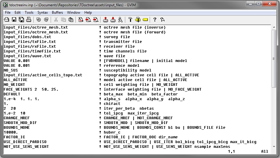
Fig. 3.4 Example input file for the inversion program (Download ). Example input file for forward modeling only (Download ).

3.2.5.1. Line Descriptions

• Inversion OcTree Mesh: file path to the OcTree mesh associated with the recovered model. All reference models, starting models and bounds should be defined on this mesh.

• Forward OcTree Mesh: file path to the OcTree mesh on which the forward problem is solved. Generally, this is defined to be the same as the inversion OcTree mesh. In the case that it is different, the current model will be interpolated from the inversion OcTree mesh to the forward OcTree mesh in order to solve the forward problem.

• Observation File: file path to the observed data file or a survey index file (forward modeling only).

• Transmitters File: file path to the transmitters file

• Receivers File: file path to the receivers file

• Time Channels File: file path to the time channels file

• Wave file: Set the path to a wave file. This file defines the time-steps for the problem.

• Initial/FWD Model: On this line we specify either the starting model for the inversion or the conductivity model for the forward modeling. On this line, there are 3 possible options:

  • If the program is being used to forward model data, the flag ‘FWDMODEL’ is entered followed by the path to the conductivity model.

  • If the program is being used to invert data, only the path to a conductivity model is required; e.g. inversion is assumed unless otherwise specified.

  • If a homogeneous conductivity value is being used as the starting model for an inversion, the user can enter “VALUE” followed by a space and a numerical value; example “VALUE 0.01”.

Important

If data are only being forward modeled, only the active topography cells and tol_bicg tol_ipcg_bicg max_it_bicg fields are relevant. However, the remaining fields must not be empty and must have correct syntax for the code to run.

• Reference Model: The user may supply the file path to a reference conductivity model. If a homogeneous conductivity value is being used for all active cells, the user can enter “VALUE” followed by a space and a numerical value; example “VALUE 0.01”.

• Susceptibility Model: The user may supply the file path to a background susceptibility model. Or the user may enter the flag NO_SUS if the background susceptibility is zero.

• Active Topography Cells: Here, the user can choose to specify the cells which lie below the surface topography. To do this, the user may supply the file path to an active cells model file or type “ALL_ACTIVE”. The active cells model has values 1 for cells lying below the surface topography and values 0 for cells lying above.

• Active Model Cells: Here, the user can choose to specify the model cells which are active during the inversion. To do this, the user may supply the file path to an active cells model file or type “ALL_ACTIVE”. The active cells model has values 1 for cells lying below the surface topography and values 0 for cells lying above. Values for inactive cells are provided by the background conductivity model.

• Cell Weights: Here, the user specifies whether cell weights are supplied. If so, the user provides the file path to a cell weights file If no additional cell weights are supplied, the user enters “NO_WEIGHT”.

• Face Weights: Here, the user specifies whether face weights are supplied. If so, the user provides the file path to a face weights file cell weights file. If no additional cell weights are supplied, the user enters “NO_FACE_WEIGHT”. The user may also enter “EKBLOM” for 1-norm approximation to recover sharper edges.

• beta_max beta_min beta_factor: Here, the user specifies protocols for the trade-off parameter (beta). beta_max is the initial value of beta, beta_min is the minimum allowable beta the program can use before quitting and beta_factor defines the factor by which beta is decreased at each iteration; example “1E4 10 0.2”. The user may also enter “DEFAULT” if they wish to have beta calculated automatically.

• alpha_s alpha_x alpha_y alpha_z: Alpha parameters . Here, the user specifies the relative weighting between the smallness and smoothness component penalties on the recovered models.

• Chi Factor: The chi factor defines the target misfit for the inversion. A chi factor of 1 means the target misfit is equal to the total number of data observations.

• iter_per_beta nBetas: Here, iter_per_beta is the number of Gauss-Newton iterations per beta value. nBetas is the number of times the inverse problem is solved for smaller and smaller trade-off parameters until it quits. See theory section for cooling schedule and Gauss-Newton update.

• tol_ipcg max_iter_ipcg: Here, the user specifies solver parameters. tol_ipcg defines how well the iterative solver does when solving for \(\delta m\) and max_iter_ipcg is the maximum iterations of incomplete-preconditioned-conjugate gradient. See theory on Gauss-Newton solve

• Reference Model Update: Here, the user specifies whether the reference model is updated at each inversion step result. If so, enter “CHANGE_MREF”. If not, enter “NOT_CHANGE_MREF”.

• Hard Constraints: SMOOTH_MOD runs the inversion without implementing a reference model (essential \(m_{ref}=0\)). “SMOOTH_MOD_DIF” constrains the inversion in the smallness and smoothness terms using a reference model.

• Bounds: Bound constraints on the recovered model. Choose “BOUNDS_CONST” and enter the values of the minimum and maximum model conductivity; example “BOUNDS_CONST 1E-6 0.1”. Enter “BOUNDS_NONE” if the inversion is unbounded, or if there is no a-prior information about the subsurface model.

• Huber constant: Here, the user may control the sparseness of the recovered model by specifying the Huber constant (\(\epsilon\)) within the Huber norm. The TDoctree code uses the Huber norm to define the smallness term (link) in the inversion. If a large value is used (default = 10000), the inversion will use an L2 norm for the smallness. If a sufficiently small value is used, the smallness will be similar to an L1 norm. The Huber norm is given by:

\[\begin{split}\sum_{i=1}^M x_i^2 \;\;\;\; \textrm{where} \;\;\;\; x_i = \begin{cases} \sigma_i^2 \;\; \textrm{for} \;\; \sigma_i \leq \epsilon \\ \epsilon \big ( 2 |\sigma_i | - \epsilon \big ) \;\; \textrm{for} \;\; \sigma_i > \epsilon \end{cases}\end{split}\]

• Memory Options: This code uses a factorization to solve the forward system at each frequency. These factorizations must be stored. By using the flag ‘FACTOR_IC’ (in cpu), factorizations are stored within a computer’s RAM. Although this is faster, larger problems cannot be solved if insufficient temporary memory is available. The factorizations are stored in permanent memory (disk) if the flag ‘FACTOR_OOC’ (out of cpu) is used followed by the path to a directory. This is slower because the program must read these files many times. The second options is ill-advised if files are being transferred over a network.

• Solver options: Here the user chooses whether the forward problem is solved using a direct or iterative solver.

  • For Pardiso solver, the flag ‘USE_DIRECT_PARDISO’ is used.

  • For the BICG iterative solver, the flag ‘USE_ITER’ is used followed by values for the parameters tol_bicg, tol_ipcg_bicg and max_it_bicg.

    • tol_bicg: relative tolerance (stopping criteria) when solver is used during forward modeling. Ideally, this number is very small (default = 1e-10).

    • tol_ipcg_bicg: relative tolerance (stopping criteria) when solver needed in computation of δm during Gauss Newton iteration. This value does not need to be as large as the previous parameter (default = 1e-5).

    • max_it_bicg: maximum number of BICG iterations (default = 100)

• Sensitivity weighting options:

  • For no sensitivity weighting, use the flag NOT_USE_SENS_WEIGHT

  • To apply sensitivity weighting, use the flag USE_SENS_WEIGHT followed by values for the parameters nsample and maxSens. If applied, sensitivity weights are constructed using the starting model and the weights used in the inversion are output to the file sensitivity.txt.

  The parameters nsample and maxSens are defined as follows:

  • nsample is the number of iterations used to approximate the root mean squares sensitivities with the probing method; see sensitivity weights. nsample corresponds to the value of the variable \(K\) in the mathematical description. Generally nsample is an integer value between 5 and 10.

  • maxSens is the maximum value for the sensitivity weights; see sensitivity weights. maxSens corresponds to the variable \(\tau\) in the mathematical description. Generally this is a number between 10 and 1000.